Hoofdstuk 4: Fourier-analyse

Ter herhaling de definite van de Fourier-getransformeerde $\hat{f}$ van een functie $f$:

$$ \hat{f}(w) = \frac{1}{\sqrt{2\pi}}\int_{-\infty}^{\infty} f(x) e^{-iwx}\,dx$$

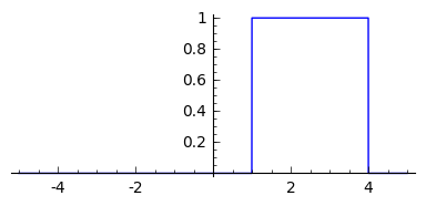
Om stukgewijze functies voor te stellen kan de identificatie functie van een interval gebruikt worden:

def I(a, b): return (sign(x-a) - sign(x-b)) /2 plot(I(1,4), (x, -5, 5), figsize=[4,2])

Oefening 1

Controleer slide 79 en 80

Bekijk de Fourier-getransformeerde (zowel formule als plot) van $f(x) = k$ als $x \in [0, a]$ anders $f(x) = 0$.

Controleer slide 82, 83 en 84

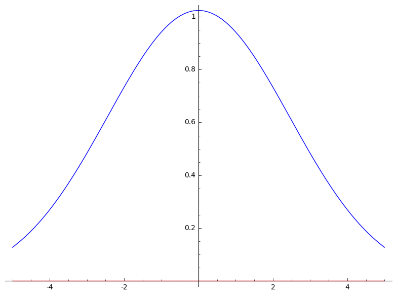
Bekijk de Fourier-getransformeerde van de Gaussiaan: $f(x) = e^{-a x^2}$.

var("a", "k") f(x) = I(0, a)*k f

$\newcommand{\Bold}[1]{\mathbf{#1}}x \ {\mapsto}\ -\frac{1}{2} \, k {\left(\mathrm{sgn}\left(-a + x\right) - \mathrm{sgn}\left(x\right)\right)}$

plot(f.subs({a: 1, k: 2}), (x, -5, 5), figsize=[5,3])

def Fourier(f): Ff(w) = integrate(f(x)*e^(-i*x*w), x, -oo, oo) return Ff

fhat = Fourier(f) fhat.subs(a=1)

$\newcommand{\Bold}[1]{\mathbf{#1}}w \ {\mapsto}\ -\frac{1}{2} \, k {\left(-\frac{2 i \, e^{\left(-i \, w\right)}}{w} + \frac{2 i}{w}\right)}$

values = { a: 1, k: 2 } plot(real(fhat.subs(values)), (w, -5, 5)) + plot(imag(fhat.subs(values)), (w, -5, 5), color="red")

values = { a: 2, k: 3 } plot(real(fhat.subs(values)), (w, -5, 5)) + plot(imag(fhat.subs(values)), (w, -5, 5), color="red")

g(x) = e^(-a*x^2) assume(a > 0) ghat = Fourier(g) forget(a > 0) ghat

$\newcommand{\Bold}[1]{\mathbf{#1}}w \ {\mapsto}\ \frac{\sqrt{\pi} e^{\left(-\frac{w^{2}}{4 \, a}\right)}}{\sqrt{a}}$

values = { a: 3 } plot(real(ghat.subs(values)), (w, -5, 5)) + plot(imag(ghat.subs(values)), (w, -5, 5), color="red")

Convolutie

Bij definitie geldt:

$$(f \otimes g)(x) = \int_{-\infty}^{\infty}f(p) g(x-p)\,dp$$

Oefening 2

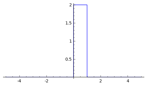
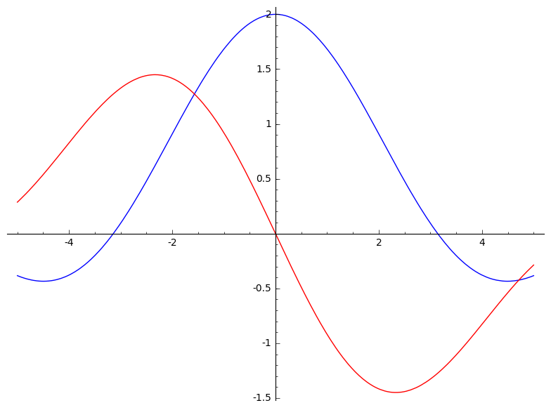
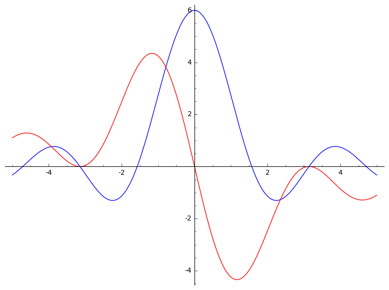
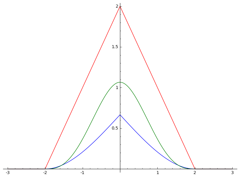
Stel $f(x)$, $g(x)$, $h(x)$, zoals in de afbeeldingen:

Bereken de convoluties met behulp van de definitie: $f \otimes f$, $g \otimes g$, $h \otimes h$, $f \otimes g$, $f \otimes h$, $g \otimes h$.

Plot ook de resultaten.

var("p") f(x) = I(-1,1)*(1+x)/2 g(x) = I(-1,1) h(x) = I(-1,1)*(1-x^2) def convolution(a, b): return integrate(a(p)*b(p-x), p, -oo, oo)

(plot(convolution(f, f), (x, -3, 3), color="blue") + plot(convolution(g, g), (x, -3, 3), color="red") + plot(convolution(h, h), (x, -3, 3), color="green"))

(plot(convolution(f, g), (x, -3, 3), color="blue") + plot(convolution(f, h), (x, -3, 3), color="red") + plot(convolution(g, h), (x, -3, 3), color="green"))

Oefening 3

Op slide 94 vinden we de convolutie stelling terug:

$$\mathcal{F}(f \otimes g) = \sqrt{2\pi}\mathcal{F}(f)\mathcal{F}(g)$$

en dus:

$$ f \otimes g = \sqrt{2\pi} \mathcal{F}^{-1}\left(\mathcal{F}(f)\mathcal{F}(g)\right)$$

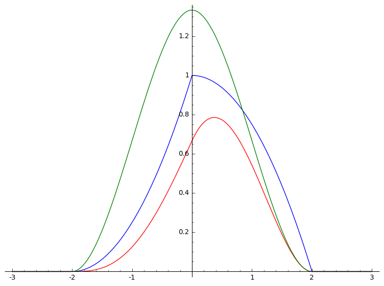
Gebruik deze stelling om de convoluties uit oefeining 2 anders te berekenen.

Sage is niet in staat om de inverse Fourierrtansformatie symbolisch uit te rekenen

[ModSim] H4 (oplossingen)